Entropy estimates in the isochrone potential
Here we estimate the entropy of samples in the isochrone potential, and plot it as a function of time while integrating orbits for these samples - see the Introduction for the general expressions.
We do that both for self-consistent and non-stationary samples. In the self-consistent case, we compare the estimates with the true entropy calculated with analytical expressions for the DF and density of states of the isochrone model. We use the agama package for the orbit integration, sampling from a DF and action calculations, but you may prefer other packages, such as gala or galpy. Of course, the entropy estimate itself does not depend on the library used to generate data and integrate orbits.
However, note that the entropy estimates assume the samples are i.i.d. (independent and identically distributed), which is generally the case for data generated with so-called pseudo random number generators (PRNG). Data generated by quasi-random number generators (QRNG) in general are significantly non i.i.d, which can produce biased entropy estimates.
We estimate the entropy of the DF \(f(\vec{w})\), where \(\vec{w} = (\vec{r}, \vec{v})\) are the 6D phase-space coordinates:
\(S \equiv -\int f(\vec{w})\ln\left(\frac{f}{\mu}\right)\, \mathrm{d}^6\vec{w} = -\int f'(\vec{w}')\ln f'\, \mathrm{d}^6\vec{w}'\),
where \(\mu = |\Sigma|^{-1}\), \(|\Sigma|\) is the product of the dispersions in each of the coordinates, and \(f'(\vec{w}') = f(\vec{w})/\mu = |\Sigma|f(\vec{w})\) is the DF of the coordinates normalized by their dispersions - see the Introduction.
Assuming that \(f(\vec{w})\) is a function of integrals \(\vec{I}\) only, e.g. \(f=f(E)\), \(f = f(E,L)\), or \(f = f(\vec{J})\) (all valid assumptions for the self-consistent sample of the isochrone model), where \(E\) is energy, \(L\) is angular momentum, and \(\vec{J}\) are three actions, with the appropriate change of variables we obtain in general
\(S_{\vec{I}} = -\int F(\vec{I}) \ln\left( \frac{|\Sigma|F(\vec{I})}{g(\vec{I})}\right)\, \mathrm{d}\vec{I}\),
where \(g(\vec{I})\) is the density of states – see Appendix A of Beraldo e Silva et al (2025) for details. Note that \(S_{\vec{I}}\) is not “the entropy in the space of integrals” but, instead, \(S_{\vec{I}}\) is still the entropy of the 6D DF \(f\), i.e. \(S_{\vec{I}} = S(f)\), for cases where one can assume that the DF is \(f = f(\vec{I})\), which is true for stationary samples (Jeans’ theorem).
The codes are essentially the same used to produce Figs. 2 and 4 in Beraldo e Silva et al (2025). For the paper, we generated samples as large as \(N=10^8\), but below we generate only up to \(N=10^6\), and one can decrease the size, or the number of time-steps where the entropy is estimated if this is taking too long (it takes a few minutes for \(N=10^6\) evaluated in 100 time-steps in a laptop).
We start importing the relevant modules and setting some parameters for prettier plots. We use agama to generate samples, integrate orbits and calculate actions, but any other libray could be used instead.
[1]:
# Import modules
import numpy as np
from scipy import integrate
import matplotlib as mpl
import matplotlib.pyplot as plt

import agama
import tropygal

from matplotlib.ticker import ScalarFormatter, NullFormatter

params = {'axes.labelsize': 24, 'xtick.labelsize': 20,
          'xtick.direction': 'in', 'xtick.major.size': 8.0,
          'xtick.bottom': 1, 'xtick.top': 1, 'ytick.labelsize': 20,
          'ytick.direction': 'in','ytick.major.size': 8.0,'ytick.left': 1,
          'ytick.right': 1,'text.usetex': True, 'lines.linewidth': 1,
          'axes.titlesize': 32, 'font.family': 'serif'}
plt.rcParams.update(params)
plt.rcParams['figure.dpi'] = 60
columnwidth = 240./72.27
textwidth = 504.0/72.27

%matplotlib inline
%config InlineBackend.figure_format = 'retina'
Set constants
[3]:
# Mass and scale radius for the isochrone potential:
M = 1.
b = 1.

# Making sure we have G = 1:
agama.setUnits()
G = agama.G
print ('G:',G)

n_steps = 100 # number of time steps in the orbit integration (and at which the entropy is estimated)

n_orbs = [int(N) for N in [1e+4, 1e+5, 1e+6]]
# For the plots:
N_label = ['10k', '100k', '1m']
N_label_plot = [r'$10^4$', r'$10^5$', r'$10^6$']
N_colors = ['black', 'red', 'blue']
G: 1.0
Define functions for true entropy of self-consistent sample
[4]:
# Analytical expressions for DF of self-consistent isochrone model:
def F_E(E, M, b, G):
    f_E = tropygal.DF_Isochrone(E, M, b, G=G)
    g_E = tropygal.g_Isochrone(E, M, b, G=G)

    return f_E*g_E # F(E) = f(E)g(E)
#-----------------
def S_E_true_integrand(E, M, b, mu, G):
    # Integrand for calculation of true entropy
    # F(E) = f(E) * g(E)
    # it returns F(E) * ln(F(E)/mu(E)), and mu(E) = |Sigma|^(-1) * g(E)
    f_E = tropygal.DF_Isochrone(E, M, b, G)

    return F_E(E, M, b, G)*np.log(f_E/mu) # externally, mu is set to |Sigma|^(-1)
Check normalization of F(E)
[5]:
E_I_min = -M*G/(2.*b) # Minimum of potential
E_I_max = -1e-7

norm = integrate.quad(F_E, a=E_I_min, b=E_I_max, args=(M, b, G))[0]
print ('norm of F(E):', norm)
norm of F(E): 0.9999996800000946
Create Isochrone model
[6]:
# Potential and DF (using agama)
# This creates an isochrone potential of a given mass and scale radius:
isoc_pot = agama.Potential(type='Isochrone', mass=M, scaleRadius=b)
# This creates a DF of a self-consistent sample:
isoc_df = agama.DistributionFunction(type='QuasiSpherical', potential=isoc_pot, density=isoc_pot)
# This creates an action finder for the given potential:
actF = agama.ActionFinder(isoc_pot)
Compare DF estimates
Knowing the analytical DF of a self-consistent sample of an isochrone model, we compare it with DF estimates in different integrals-of-motion spaces.
The DF at a point \(i\) is estimated with the function tropygal.density() as \(\hat{f}_i = \frac{e^{\psi(k)}}{(N-1)V_d {D_{ik}}^d}\), where \(k\) is the k-th neighbor, \(V_d\) is the volume of the unit-radius hypershpere, \(D_{ik}\) is the distance to the k-th neighbor and \(d\) is the dimension – see e.g. Leonenko, Pronzato & Savani 2008. Note that this density estimate is specifically tuned as a plugin density in an entropy estimate, such that this has zero bias and variance for \(N\rightarrow \infty\). So, this is not necessarily the best density estimate per se, but it has been shown to produce consistent entropy estimates.
[7]:
nbins_E = 10_000 # number of energy bins for the analytic DF
N = n_orbs[0] # number of sampling points

bin_edges_E = np.linspace(E_I_min, E_I_max, nbins_E+1)
bins_E = 0.5*(bin_edges_E[:-1] + bin_edges_E[1:])

f_E_true = tropygal.DF_Isochrone(bins_E, M, b, G)

# Generate self-consistent sample of the isochrone potential.
# Some care is needed here, since it's important to make sure the initial sample is really stationary in the potential.
# A constant entropy for this sample indicates that it is truly stationary - see plot below with the time evolution.
# The entropy estimates assume the samples are i.i.d. (independent and identically distributed).
# This is generally true for a sample generated with a pseudo random number generator (PRNG), but not true for a quasi random (QRNG) method.
# If using agama, see option #define DISABLE_QRNG in src/math_sample.cpp, or in Makefile.local, which might need to be set before compilation.

data,_ = agama.GalaxyModel(isoc_pot, isoc_df).sample(N)
# data, _ = isoc_pot.sample(N, potential=isoc_pot)
#------------------------------
sigma_6D = np.array([0.5*(np.percentile(coord, 84) - np.percentile(coord, 16)) for coord in data.T])
x  = data[:,0]; y  = data[:,1]; z  = data[:,2]
vx = data[:,3]; vy = data[:,4]; vz = data[:,5]

# DF estimates in 6D:
f_6D_hat_k1 = (1./np.prod(sigma_6D))*tropygal.density(data/sigma_6D, k=1)
f_6D_hat_k10 = (1./np.prod(sigma_6D))*tropygal.density(data/sigma_6D, k=10, correct_bias=False)
f_6D_hat_k10_correc = (1./np.prod(sigma_6D))*tropygal.density(data/sigma_6D, k=10, correct_bias=True)

v2 = vx**2 + vy**2 + vz**2
pos = np.column_stack((x, y, z))
E = isoc_pot.potential(pos) + 0.5*v2
sigma_E = 0.5*(np.percentile(E, 84) - np.percentile(E, 16))
g_E = np.sqrt(sigma_E)*tropygal.g_Isochrone(E/sigma_E, M/sigma_E, b, G=G)

# DF estimates in energy space
f_E_hat_k1 = (1./sigma_E)*tropygal.density(E/sigma_E, k=1)/g_E
f_E_hat_k10 = (1./sigma_E)*tropygal.density(E/sigma_E, k=10)/g_E
#--------------------------

Lx = (y*vz - z*vy)
Ly = (z*vx - x*vz)
Lz = (x*vy - y*vx)
L = np.sqrt(Lx**2 + Ly**2 + Lz**2)
EL = np.column_stack((E, L))
sigma_L = 0.5*(np.percentile(L, 84) - np.percentile(L, 16))
sigma_EL = np.array([sigma_E, sigma_L])

# g_EL = (sigma_L**2/sigma_E)*tropygal.gEL_Isochrone(E/sigma_E, L/sigma_L, M/(sigma_L*np.sqrt(sigma_E)), G=G)
g_EL = tropygal.gEL_Isochrone(E, L, M, G=G)

# DF estimates in energy-angular momentum space
f_EL_hat_k1 = (1./np.prod(sigma_EL))*tropygal.density(EL/sigma_EL, k=1)/g_EL
f_EL_hat_k10 = (1./np.prod(sigma_EL))*tropygal.density(EL/sigma_EL, k=10)/g_EL
#----------------

J = actF(data, actions=True, frequencies=False, angles=False)
sigma_J = np.array([0.5*(np.percentile(coord, 84) - np.percentile(coord, 16)) for coord in J.T])

# DF estimates in action space
f_J_hat_k1 = (1./np.prod(sigma_J))*tropygal.density(J/sigma_J, k=1)/(2*np.pi)**3
f_J_hat_k10 = (1./np.prod(sigma_J))*tropygal.density(J/sigma_J, k=10)/(2*np.pi)**3
[8]:
fig, axs = plt.subplots(1, 3, figsize=(24, 7))
fig.patch.set_facecolor('white')
fig.suptitle('Isochrone Model (self-consistent)', fontsize=36)

titles = ['E-space', '(E,L)-space', r'$(\vec{J})$-space']
ylabels = ['Distribution Function', None, None]
ylabels_pos = [True, False, False]

# Data for scatter plots
scatter_data = [(E, f_E_hat_k1, r'$\hat{f}(E) = \hat{F}(E)/g(E)$'),
                (E, f_EL_hat_k1, r'$\hat{f}(E,L) = \hat{F}(E,L)/g(E,L)$'),
                (E, f_J_hat_k1, r'$\hat{f}(\vec{J}) = \hat{F}(\vec{J})/(2\pi)^3$')
]
scatter_red_data = [(E, f_E_hat_k10),
                    (E, f_EL_hat_k10),
                    (E, f_J_hat_k10)]
# Create subplots
for i, ax in enumerate(axs):
    ax.set_title(titles[i])

    # Scatter grey (k=1)
    sc_grey = ax.scatter(*scatter_data[i][:2], s=10, marker='.', facecolor='grey',
                         edgecolor='none', alpha=0.7, label=scatter_data[i][2])
    # Scatter red (k=10)
    sc_red = ax.scatter(*scatter_red_data[i], s=10, marker='.', facecolor='red',
                        edgecolor='none', alpha=0.3, label=r'$k=10$')
    # Analytic curve
    line_analytic, = ax.plot(bins_E, f_E_true, 'k-', lw=2, zorder=0, label=r'$f(E)$ -- analytic')

    # Axes formatting
    ax.set_yscale('log')
    ax.set_ylim(1e-12, 1)
    ax.set_xlabel(r'$E$', fontsize=30)
    if ylabels_pos[i]:
        ax.set_ylabel(ylabels[i], fontsize=30)
    else:
        ax.tick_params(labelleft=False)

    # First legend:
    legend1 = ax.legend(handles=[sc_grey, line_analytic], fontsize=30, markerscale=5)
    ax.add_artist(legend1)

# Second legend:
legend2 = axs[0].legend(handles=[sc_grey, sc_red], labels=[r'$k=1$', r'$k=10$'],
                    fontsize=30, markerscale=5, loc='center left')

fig.subplots_adjust(left=0.05, right=0.95, top=0.825, bottom=0.07, wspace=0.05)
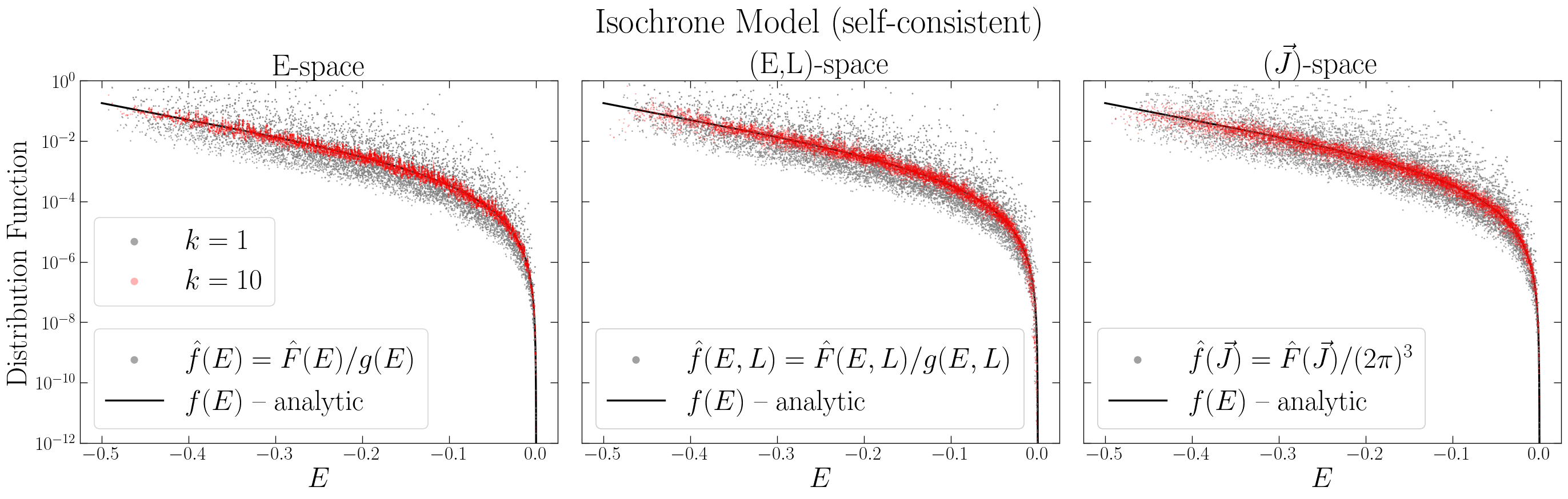
We see that the DF is very well estimated in these low dimensional spaces of integrals of motion.
Increasing the kth neighbor used in the estimate (red) substancially decreases the scatter.
Below we plot the DF estimates in 6D.
[9]:
fig, axs = plt.subplots(1, 3, figsize=(24, 7))
fig.patch.set_facecolor('white')
fig.suptitle('Isochrone Model (self-consistent)', fontsize=36)

titles = [r'$k=1$', r'$k=10$', r'$k=1$ (bias corrected)']
ylabels = ['Distribution Function', None, None]
ylabels_pos = [True, False, False]
colors = ['grey', 'red', 'red']

# Data for scatter plots
scatter_data = [(E, f_6D_hat_k1, r'$\hat{f}(\vec{w})$'),
                (E, f_6D_hat_k10, r'$\hat{f}(\vec{w})$'),
                (E, f_6D_hat_k10_correc, r'$\hat{f}(\vec{w})$')
]

# Create subplots
for i, ax in enumerate(axs):
    ax.set_title(titles[i])

    # Scatter grey (k=1)
    sc_grey = ax.scatter(*scatter_data[i][:2], s=10, marker='.', facecolor=colors[i],
                         edgecolor='none', alpha=0.5, label=scatter_data[i][2])
    # Analytic curve
    line_analytic, = ax.plot(bins_E, f_E_true, 'k-', lw=2, zorder=0, label=r'$f(E)$ -- analytic')

    # Axes formatting
    ax.set_yscale('log')
    ax.set_ylim(1e-12, 1)
    ax.set_xlabel(r'$E$', fontsize=30)
    if ylabels_pos[i]:
        ax.set_ylabel(ylabels[i], fontsize=30)
    else:
        ax.tick_params(labelleft=False)

    legend1 = ax.legend(handles=[sc_grey, line_analytic], fontsize=30, markerscale=5)

fig.subplots_adjust(left=0.05, right=0.95, top=0.825, bottom=0.07, wspace=0.05)
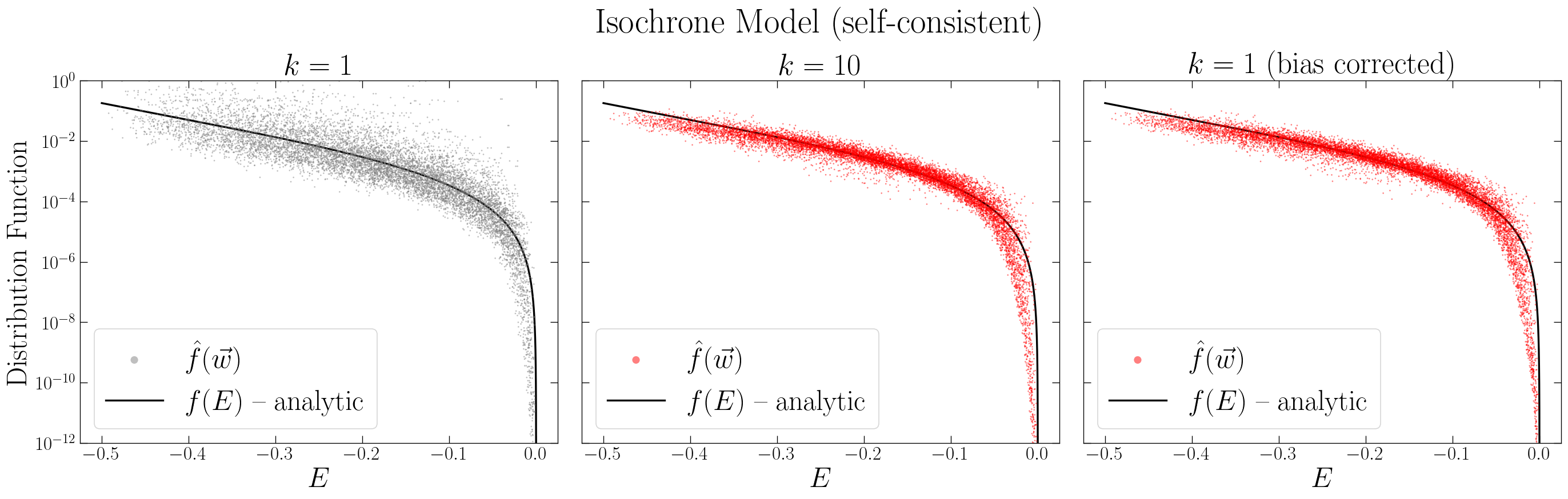
Overall we still have reasonable DF estimates, with increasing k decrasing the scatter. But for a fixed number of sampling points, in a higher dimensional space it is harder to estimate the density, in comparison to the estimates in lower dimensions made before. The bias correction slightly improves the estimates for points at the high-energy (low-DF) tail.
Estimate entropy
Note that, while above we were showing the DF \(f\), below we will compare estimates of the entropy of the DF of the normalized coordinates, i.e. the entropy of \(f' = |\Sigma_0|f\), where \(|\Sigma_0|\) is the product of the initial dispersions of the 6d coordinates.
[11]:
# Set params and initialize arrays:
kNN = 1 # which Nearest Neighbor

Tcirc = np.full(len(n_orbs), np.nan) # mean circular period for each sample
t = np.full((len(n_orbs), n_steps), np.nan) # time in the orbit integration

S_E_true = np.full(len(n_orbs), np.nan)
S_6D = np.full((len(n_orbs), n_steps), np.nan) # Entropy evaluated in 6D

# Entropies assuming the DF is f = f(E), or f = f(E,L), or f = f(J)
# These should be the same as S_6D if f = f(E), or f = f(E,L), or f = f(J)
S_E = np.full(len(n_orbs), np.nan)
S_EL = np.full(len(n_orbs), np.nan)
S_J = np.full(len(n_orbs), np.nan)
[12]:
# Generate samples, integrate and estimate entropy:
for i in range(len(n_orbs)):
    print ('-------------------------')
    dim = 6
    print ('Generating sample...')
    N = n_orbs[i]
    # Generate self-consistent sample of the isochrone potential.
    # Some care is needed here, since it's important to make sure the initial sample is really stationary in the potential.
    # A constant entropy for this sample indicates that it is truly stationary - see plot below with the time evolution.
    # If using agama, see option #define DISABLE_QRNG in src/math_sample.cpp, or in Makefile.local, which might need to be set before compilation
    if (i>0): # just to re-use the sample for generated before for N=10^4
        data,_ = agama.GalaxyModel(isoc_pot, isoc_df).sample(N)
    # data, _ = isoc_pot.sample(N, potential=isoc_pot)
    #------------------------------
    sigma_6D_0 = np.array([0.5*(np.percentile(coord, 84) - np.percentile(coord, 16)) for coord in data.T])
    mu_0 = 1./np.prod(sigma_6D_0)

    # In principle, S_true shouldn't depend on the sample size, and could be calculated outside of this loop,
    # But we are using mu = |Sigma|^(-1) to normalize the coordinates, with the exact |Sigma| changing for different samples,
    # but |Sigma| converges for large samples
    S_E_true[i] = -integrate.quad(S_E_true_integrand, a=E_I_min, b=E_I_max, args=(M, b, mu_0, G))[0]
    print ('S_E (true):', np.round(S_E_true[i], 5))
    #------------------------------
    # Estimate S_6D (at t=0; estimates over time are done below):
    S_6D[i, 0] = tropygal.entropy(data/sigma_6D_0, k=kNN)
    print ('S_6D estimated:', np.round(S_6D[i, 0], 5))
    #------------------
    # Estimate S_E, i.e. assuming f = f(E):

    x  = data[:,0]; y  = data[:,1]; z  = data[:,2]
    vx = data[:,3]; vy = data[:,4]; vz = data[:,5]

    v2 = vx**2 + vy**2 + vz**2
    pos = np.column_stack((x, y, z))
    E = isoc_pot.potential(pos) + 0.5*v2
    sigma_E = 0.5*(np.percentile(E, 84) - np.percentile(E, 16))

    g_E = tropygal.g_Isochrone(E, M, b=b, G=G)
    # It's convenient to normalize coordinates in the space where the entropy is estimated,
    # but we want to stick to the entropy definition we used before, so the normalized coordinates are passed as the data,
    # and mu takes care of the appropriate factors in the change of variables for the integral defining the entropy to be the same.
    S_E[i] = tropygal.entropy(E/sigma_E, mu= g_E*sigma_E*mu_0, k=kNN)
    print ('S_E estimated:', np.round(S_E[i], 5))
    #-------------------------
    # Estimate S_EL, i.e. assuming f = f(E,L):

    Lx = (y*vz - z*vy)
    Ly = (z*vx - x*vz)
    Lz = (x*vy - y*vx)
    L = np.sqrt(Lx**2 + Ly**2 + Lz**2)
    EL = np.column_stack((E, L))
    sigma_L = 0.5*(np.percentile(L, 84) - np.percentile(L, 16))
    sigma_EL = np.array([sigma_E, sigma_L])

    g_EL = tropygal.gEL_Isochrone(E, L, M, G=G)
    S_EL[i] = tropygal.entropy(EL/sigma_EL, mu= g_EL*np.prod(sigma_EL)*mu_0, k=kNN)
    print ('S_EL estimated:', np.round(S_EL[i], 5))
    #------------------------------
    # Estimate S_J, i.e. assuming f = f(J):

    J = actF(data, actions=True, frequencies=False, angles=False)
    sigma_J = np.array([0.5*(np.percentile(coord, 84) - np.percentile(coord, 16)) for coord in J.T])
    S_J[i] = tropygal.entropy(J/sigma_J, mu= ((2.*np.pi)**3)*np.prod(sigma_J)*mu_0, k=kNN)
    print ('S_J estimated:', np.round(S_J[i],5))
    #------------------------------
    # Estimate S_6D at different times

    # define integration time (same for all orbits):
    Tcirc[i] = np.median(isoc_pot.Tcirc(data))
    int_time = 50*Tcirc[i]
    delta_t = int_time/n_steps

    # Integrate orbits for the entire time interval, storing the outputs at regular timesteps:
    orbs = agama.orbit(potential=isoc_pot, ic=data, time=int_time, trajsize=n_steps, method='dop853', accuracy=1e-6, verbose=False)
    # Other orbit integration methods:
    #orbs = agama.orbit(potential=isoc_pot, ic=data, time=int_time, trajsize=n_steps, method='dprkn8', accuracy=1e-6, verbose=False)
    t[i] = orbs[0,0]  # 0th column is the array of times for each orbit (identical for all orbits, so we take the one from the 0th row)
    trajs = np.stack(orbs[:,1])  # 1st column is the array of trajectories, each element is itself a N x 6 array; stack them up.
    for j in range(1, n_steps):
        all_coords = trajs[:,j]
        sigma_6D = np.array([0.5*(np.percentile(coord, 84) - np.percentile(coord, 16)) for coord in all_coords.T])
        # Here we re-normalize again at every time-step (to facilitate the estimate),
        # "compensating" for that in the mu factor, i.e. making an appropriate change of variables every time-step:
        S_6D[i,j] = tropygal.entropy(all_coords/sigma_6D, mu=np.prod(sigma_6D)*mu_0, k=kNN)
        if (j%10==0):
            print ('j:', j, 'S_6D estimated:', np.round(S_6D[i, j], 5))
-------------------------
Generating sample...
S_E (true): 9.23354
S_6D estimated: 9.60372
S_E estimated: 9.25726
S_EL estimated: 9.27627
S_J estimated: 9.28593
j: 10 S_6D estimated: 9.58327
j: 20 S_6D estimated: 9.59528
j: 30 S_6D estimated: 9.65665
j: 40 S_6D estimated: 9.60824
j: 50 S_6D estimated: 9.62535
j: 60 S_6D estimated: 9.63396
j: 70 S_6D estimated: 9.62389
j: 80 S_6D estimated: 9.62115
j: 90 S_6D estimated: 9.66882
-------------------------
Generating sample...
S_E (true): 9.25089
S_6D estimated: 9.50836
S_E estimated: 9.25667
S_EL estimated: 9.26148
S_J estimated: 9.26284
j: 10 S_6D estimated: 9.50923
j: 20 S_6D estimated: 9.51431
j: 30 S_6D estimated: 9.50902
j: 40 S_6D estimated: 9.50916
j: 50 S_6D estimated: 9.5049
j: 60 S_6D estimated: 9.50605
j: 70 S_6D estimated: 9.50404
j: 80 S_6D estimated: 9.51362
j: 90 S_6D estimated: 9.51055
-------------------------
Generating sample...
S_E (true): 9.25154
S_6D estimated: 9.42569
S_E estimated: 9.25121
S_EL estimated: 9.25654
S_J estimated: 9.25798
j: 10 S_6D estimated: 9.42512
j: 20 S_6D estimated: 9.42568
j: 30 S_6D estimated: 9.42483
j: 40 S_6D estimated: 9.42685
j: 50 S_6D estimated: 9.42477
j: 60 S_6D estimated: 9.42179
j: 70 S_6D estimated: 9.42349
j: 80 S_6D estimated: 9.4241
j: 90 S_6D estimated: 9.42064
Plot
[13]:
# Calc errors
err_S_6D = np.zeros(len(n_orbs))
err_S_E = np.zeros(len(n_orbs))
err_S_EL = np.zeros(len(n_orbs))
err_S_J = np.zeros(len(n_orbs))
#-------------------
for i in range(len(n_orbs)):
    # Calculate error with the time-average of S_6D, in respect to the true value:
    err_S_6D[i] = (np.mean(S_6D[i]) - S_E_true[-1])/S_E_true[-1]

    err_S_E[i] = (S_E[i] - S_E_true[-1])/S_E_true[-1]
    err_S_EL[i] = (S_EL[i] - S_E_true[-1])/S_E_true[-1]
    err_S_J[i] = (S_J[i] - S_E_true[-1])/S_E_true[-1]

    print ('N:', n_orbs[i],'S_E_true:', S_E_true[-1], 'err S_J:',(np.mean(S_J[i]) - S_E_true[-1]))
N: 10000 S_E_true: 9.251537903193213 err S_J: 0.034393275767982345
N: 100000 S_E_true: 9.251537903193213 err S_J: 0.011298802203482339
N: 1000000 S_E_true: 9.251537903193213 err S_J: 0.006439728862449812
[14]:
# Plot
fig, axs = plt.subplots(2, 1, figsize=(8,14))
fig.patch.set_facecolor('white')

axs[0].set_title('Isochrone Model (self-consistent)')
axs[1].set_title('Relative error (bias)')

ones = np.ones(n_steps)

for i in range(len(n_orbs)):
    axs[0].plot(t[i]/Tcirc[i], S_6D[i], ls='-', lw=2, c=N_colors[i], label=N_label_plot[i]) # Assumption-free estimate
    #axs[0].plot(t[i]/Tcirc[i], S_E[i]*ones, ls='--', dashes=(8,5), lw=2, c=N_colors[i]) # Assuming the DF is an unknown f = f(E)
    #axs[0].plot(t[i]/Tcirc[i], S_EL[i]*ones, ls='--', dashes=(8,5), lw=2, c=N_colors[i]) # Assuming the DF is an unknown f = f(E,L)
    axs[0].plot(t[i]/Tcirc[i], S_J[i]*ones, ls='--', dashes=(8,5), lw=2, c=N_colors[i]) # Assuming the DF is an unknown f = f(J)

# To have two legends:
l1 = axs[0].legend(fontsize=24)

p1, = axs[0].plot(t[0]/Tcirc[0], S_6D[0], ls='-', lw=2, c=N_colors[0])
p2, = axs[0].plot(t[0]/Tcirc[0], S_J[0]*ones, color=N_colors[0], linestyle='--', dashes=(8,5), lw=2)
p3, = axs[0].plot(t[-1]/Tcirc[-1], S_E_true[-1]*ones, color='grey', linestyle='-', lw=4, zorder=0)
axs[0].legend([p1, p2, p3], [r'$\hat{S}_\mathrm{6D}$', r'$\hat{S}_{\vec{J}}$', r'$S_{\mathrm{E, true}}$'],
              loc='upper left', fontsize=24)
# Add l1 as a separate artist to the axes
axs[0].add_artist(l1)
#----------------
axs[1].plot(n_orbs, np.abs(err_S_6D),'h-',c='grey', ms=15, lw=2, mec='black', alpha=0.6, label=r'$\hat{S}_\mathrm{6D}$')
axs[1].plot(n_orbs, np.abs(err_S_J), '^--', c='grey', ms=15, dashes=(8,5), lw=2, mec='black', alpha=0.6, label=r'$\hat{S}_{\vec{J}}$')
axs[1].plot(n_orbs, np.abs(err_S_EL), 'x-.', c='grey', ms=15, lw=2, mec='black', alpha=0.6, label=r'$\hat{S}_\mathrm{EL}$')
axs[1].plot(n_orbs, np.abs(err_S_E), '.:', c='grey', ms=20, lw=2, mec='black', alpha=0.6, label=r'$\hat{S}_\mathrm{E}$')

axs[1].legend(fontsize=26, loc='lower left', ncol=2)
#---------------------
axs[0].set_xlabel(r'$t/T_\mathrm{circ}$')
axs[0].set_ylabel(r'$\hat{S}$')
axs[0].set_ylim(9.2,10.2)
axs[0].set_xlim(0, 50)

axs[1].set_xscale('log')
axs[1].set_yscale('log')

axs[1].set_xlabel(r'$N$')
axs[1].set_ylim(1e-5,1e-1)
axs[1].set_ylabel(r'$|\delta S|/S_{\mathrm{E, true}}$')

plt.tight_layout()
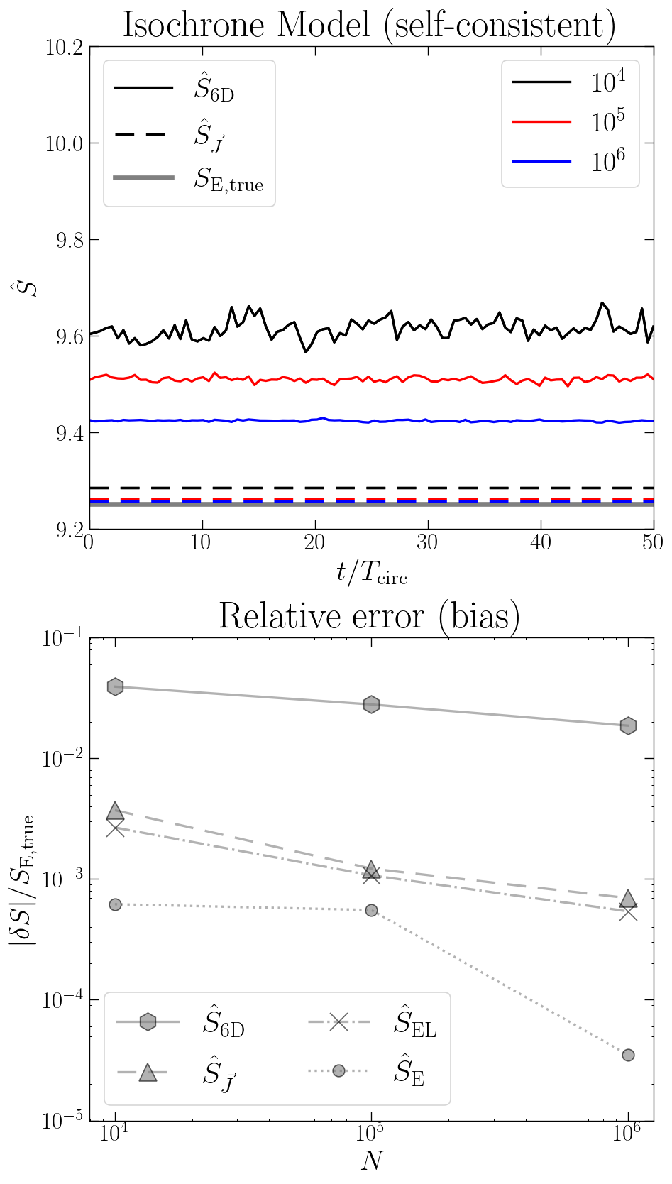
The bias is larger in higher dimensions, due to the “curse of dimensionality”: for a fixed number of sampling points, it is increasingly hard to densely populate spaces of higher dimensions. So, for a fixed number of points and increasing the dimensionality, the dataset becomes sparser. The bias is mostly due to points near the edges of the support of the distribution, and it is larger in higher dimensions because the ratio Surface/Volume is higher. In fact, the volume of an unit-radius hyper-sphere is \(V_d = \frac{\pi^{d/2}}{\Gamma\!\left( \frac{d}{2} + 1 \right)}\), and its surface area is \(A_d = \frac{2\pi^{d/2}}{\Gamma\!\left( \frac{d}{2} \right)}\), thus \(A_d/V_d = d\). In other words, in higher dimensions we have “more surface area” and a higher bias.
Evolve initial sample in new potential
[15]:
M_new = 3. # mass of new potential (where we integrate orbits for a non-stationary sample)
Now we generate the same initial sample, self-consistent with the isochrone potential of \(M=1\), but evolve the sample in an isochrone potential with mass M = 3.
After the sample phase-mixes, it will be described by a DF \(f = f(E,L)\), or \(f = f(\vec{J})\), but we can’t assume \(f = f(E)\) for the final sample, since this is anisotropic in the velocities. Since the final \(f(E,L)\) is unknown, we don’t know the exact final entropy, but this can be assumed to be \(\hat{S}_\mathrm{EL}\) for the largest sample, since we showed above that \(\hat{S}_\mathrm{EL}\) is only biased by less than \(0.1\%\).
[16]:
# Set params and initialize arrays:

Tcirc_new = np.full(len(n_orbs), np.nan) # mean circular period for each sample
t_new = np.full((len(n_orbs), n_steps), np.nan) # time in the orbit integration
S_6D_new = np.full((len(n_orbs), n_steps), np.nan) # Entropy evaluated in 6D

# Entropies assuming the DF is f = f(E,L), or f = f(J) - now only expected to be valid after the system phase-mixes
# These should be the same as S_6D if f = f(E,L), or f = f(J). In the current case, this happens at the late times only.

S_EL_new = np.full(len(n_orbs), np.nan)
S_J_new = np.full(len(n_orbs), np.nan)

# new Potential:
isoc_pot_new = agama.Potential(type='Isochrone', mass=M_new, scaleRadius=b)
# Action finder in the new potential:
actF_new = agama.ActionFinder(isoc_pot_new)
[17]:
# Same as before, but generating a sample stationary in the potential with mass M=1, and evolving it in a potential with mass M=3.
# Generate samples, integrate and estimate entropy:
for i in range(len(n_orbs)):
    print ('-------------------------')
    dim = 6
    print ('Generating sample...')
    N = n_orbs[i]
    data,_ = agama.GalaxyModel(isoc_pot, isoc_df).sample(N)
    # data, _ = isoc_pot.sample(N, potential=isoc_pot)
    sigma_6D_0 = np.array([0.5*(np.percentile(coord, 84) - np.percentile(coord, 16)) for coord in data.T])
    mu_0 = 1./np.prod(sigma_6D_0)
    #------------------------------
    # Estimate S_6D (at t=0; estimates over time are done below):

    S_6D_new[i, 0] = tropygal.entropy(data/sigma_6D_0)
    print ('S_6D estimated:', np.round(S_6D_new[i, 0], 5))
    #------------------
    # Estimate S_EL, i.e. assuming f = f(E,L):

    x  = data[:,0]; y  = data[:,1]; z  = data[:,2]
    vx = data[:,3]; vy = data[:,4]; vz = data[:,5]

    v2 = vx**2 + vy**2 + vz**2
    pos = np.column_stack((x, y, z))
    E = isoc_pot_new.potential(pos) + 0.5*v2
    sigma_E = 0.5*(np.percentile(E, 84) - np.percentile(E, 16))

    Lx = (y*vz - z*vy)
    Ly = (z*vx - x*vz)
    Lz = (x*vy - y*vx)
    L = np.sqrt(Lx**2 + Ly**2 + Lz**2)
    EL = np.column_stack((E, L))
    sigma_L = 0.5*(np.percentile(L, 84) - np.percentile(L, 16))
    sigma_EL = np.array([sigma_E, sigma_L])

    g_EL = tropygal.gEL_Isochrone(E, L, M_new, G=G)
    # It's convenient to normalize coordinates in the space where the entropy is estimated,
    # but we want to stick to the entropy definition we used before, so the normalized coordinates are passed as the data,
    # and mu takes care of the appropriate factors in the change of variables for the integral defining the entropy to be the same:
    S_EL_new[i] = tropygal.entropy(EL/sigma_EL, mu= g_EL*np.prod(sigma_EL)*mu_0)
    print ('S_EL estimated:', np.round(S_EL_new[i], 5))
    #------------------------------
    # Estimate S_J, i.e. assuming f = f(J):

    J = actF_new(data, actions=True, frequencies=False, angles=False)
    sigma_J = np.array([0.5*(np.percentile(coord, 84) - np.percentile(coord, 16)) for coord in J.T])

    S_J_new[i] = tropygal.entropy(J/sigma_J, mu= ((2.*np.pi)**3)*np.prod(sigma_J)*mu_0)
    print ('S_J estimated:', np.round(S_J_new[i],5))
    #------------------------------
    # Estimate S_6D at different times

    # define integration time (same for all orbits):
    Tcirc_new[i] = np.median(isoc_pot_new.Tcirc(data))
    int_time = 50*Tcirc_new[i]
    delta_t = int_time/n_steps

    orbs = agama.orbit(potential=isoc_pot_new, ic=data, time=int_time, trajsize=n_steps, method='dop853', accuracy=1e-6, verbose=False)
    # Other orbit integration methods:
    #orbs = agama.orbit(potential=isoc_pot_new, ic=data, time=int_time, trajsize=n_steps, method='dprkn8', accuracy=1e-6, verbose=False)
    t_new[i] = orbs[0,0]
    trajs = np.stack(orbs[:,1])
    for j in range(1, n_steps):
        all_coords = trajs[:,j]

        sigma_6D = np.array([0.5*(np.percentile(coord, 84) - np.percentile(coord, 16)) for coord in all_coords.T])
        # Here we re-normalize again at every time-step (to facilitate the estimate),
        # "compensating" for that in the mu factor, i.e. making an appropriate change of variables every time-step:
        S_6D_new[i,j] = tropygal.entropy(all_coords/sigma_6D, mu=np.prod(sigma_6D)*mu_0)
        if (j%10==0):
            print ('j:', j, 'S_6D estimated:', np.round(S_6D_new[i, j], 5))
-------------------------
Generating sample...
S_6D estimated: 9.67761
S_EL estimated: 9.8514
S_J estimated: 9.86915
j: 10 S_6D estimated: 10.26778
j: 20 S_6D estimated: 10.24959
j: 30 S_6D estimated: 10.25178
j: 40 S_6D estimated: 10.27876
j: 50 S_6D estimated: 10.27179
j: 60 S_6D estimated: 10.25475
j: 70 S_6D estimated: 10.23266
j: 80 S_6D estimated: 10.25667
j: 90 S_6D estimated: 10.2801
-------------------------
Generating sample...
S_6D estimated: 9.50951
S_EL estimated: 9.81312
S_J estimated: 9.82143
j: 10 S_6D estimated: 10.09178
j: 20 S_6D estimated: 10.10358
j: 30 S_6D estimated: 10.09785
j: 40 S_6D estimated: 10.08665
j: 50 S_6D estimated: 10.08721
j: 60 S_6D estimated: 10.07905
j: 70 S_6D estimated: 10.08552
j: 80 S_6D estimated: 10.08171
j: 90 S_6D estimated: 10.09575
-------------------------
Generating sample...
S_6D estimated: 9.42018
S_EL estimated: 9.80942
S_J estimated: 9.8111
j: 10 S_6D estimated: 9.95287
j: 20 S_6D estimated: 9.9913
j: 30 S_6D estimated: 9.99772
j: 40 S_6D estimated: 9.99939
j: 50 S_6D estimated: 9.99762
j: 60 S_6D estimated: 9.99166
j: 70 S_6D estimated: 9.99714
j: 80 S_6D estimated: 9.99317
j: 90 S_6D estimated: 9.99224
Plot
[18]:
# Plot
fig, axs = plt.subplots(2, 1, figsize=(8,14))
fig.patch.set_facecolor('white')
axs[0].set_title(r'Isochrone Model: $M_\mathrm{ini}=1$; $M_\mathrm{pot}=3$')
axs[1].set_title('Entropy variation')

ones = np.ones(n_steps)
axs[0].axhline(y=S_EL_new[-1], color='grey', linestyle='-', lw=4, zorder=0)#, label=r'$S_{EL}$')

for i in range(len(n_orbs)):
    axs[0].plot(t_new[i]/Tcirc_new[i], S_6D_new[i], ls='-', lw=2, c=N_colors[i])
    axs[0].plot(t_new[i]/Tcirc_new[i], S_J_new[i]*ones, ls='--', dashes=(8,5), lw=2, c=N_colors[i])

p4, = axs[0].plot(t_new[-1]/Tcirc_new[-1], S_EL_new[-1]*ones, color='grey', ls='-', lw=4, zorder=0)

axs[0].legend([p1, p2, p4], [r'$\hat{S}_\mathrm{6D}$', r'$\hat{S}_{\vec{J}}$', r'$\hat{S}_{\mathrm{EL, true}}$'],
              loc = 'lower left', fontsize=24)
#---------------------
# inset axes:
x1, x2, y1, y2 = 35, 49.5, 9.795, 9.855  # subregion of the original image
axins = axs[0].inset_axes([0.51, 0.1, 0.43, 0.3],
    xlim=(x1, x2), ylim=(y1, y2), xticklabels=[])#, yticklabels=[])
axins.axhline(y=S_EL_new[-1], color='grey', linestyle='-', lw=4, zorder=0)
for i in range(len(n_orbs)):
    axins.plot(t_new[i]/Tcirc_new[i], S_J_new[i]*ones, ls='--', dashes=(8,5), lw=2, c=N_colors[i])

axs[0].indicate_inset_zoom(axins, edgecolor="black")
#---------------------
# We take the final S_EL (estimated with the largest sample) as the true final S_EL:
axs[1].axhline(y=S_EL_new[-1] - S_E_true[-1],
               color='grey', linestyle='-', lw=4, label=r'$\Delta S_\mathrm{true} = \hat{S}_{\mathrm{EL, true}} - S_{\mathrm{E, true}}$')

for i in range(len(n_orbs)):
    axs[1].plot(t_new[i]/Tcirc_new[i], S_6D_new[i]-S_6D_new[i, 0], ls='-', lw=2, c=N_colors[i], label=N_label_plot[i]) # Plotting Delta S

axs[0].set_ylabel(r'$\hat{S}$')
axs[0].set_ylim(9.2, 10.3)
axs[1].set_ylabel(r'$\hat{S}_\mathrm{6D}(t) - \hat{S}_\mathrm{6D}(0)$')
axs[1].set_ylim(0, 0.65)
axs[1].legend(fontsize=24)

for i in range(2):
    axs[i].set_xlim(0, 50)
    axs[i].set_xlabel(r'$t/T_\mathrm{circ}$')

plt.tight_layout()
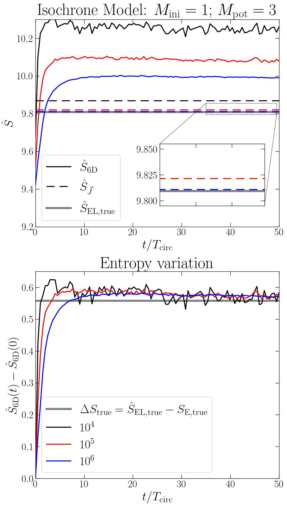
We conclude that the entropy estimate in 6D is biased by a few percent both in respect to the true initial value (as demonstrated in the plot for the self-consistent sample), and in respect to the true final value \(S_\mathrm{EL, true}\). This bias is nearly canceled by calculating entropy variations.
Besides that, not surprisingly the entropy estimates in lower dimensions, i.e. in the space of integrals, are much less biased.