Minimum-entropy fit of the isochrone potential
Here we fit a gravitational potential of the isochrone model using the kinematics of a sample in equilibrium in the correct potential, but without assuming any functional form for the tracers’ distribution function (DF). It only assumes that the DF is a function of actions evaluated in each trial potential. The correct potential is recovered as the one with minimum entropy. The physical basis of the method is explained in Beraldo e Silva et al. (2025).
This code uses the agama package to generate an equilibrium sample and to estimate the potential and action-variables, but any other library, such as gala or galpy, or personal code could be used for these tasks instead.
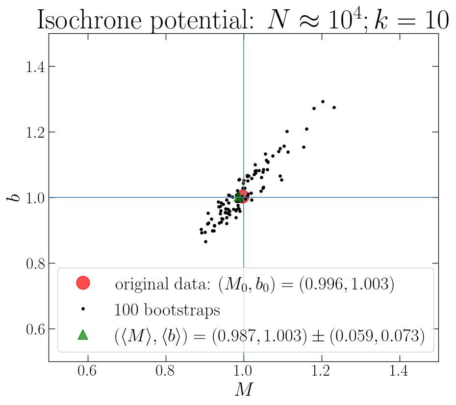
It fits the potential based on the original dataset and then later fits for a number of bootstrap samples. At the end, it shows the results based on the single (original) dataset, on each bootstrap sample and on averaging over all datasets. The plot gives an indication of how the log-likelihood surface would look like around the best if the correct functional form of the DF were specified (and then one would have a bona fide log-likelihood, which is not the case here since no DF is assumed).
[1]:
import numpy as np
from scipy import optimize
import matplotlib.pyplot as plt
plt.rcParams['figure.dpi'] = 60
import tropygal
import agama

from matplotlib.ticker import ScalarFormatter, NullFormatter

params = {'axes.labelsize': 24,
          'xtick.labelsize': 20,
          'xtick.direction': 'in',
          'xtick.major.size': 8.0,
          'xtick.bottom': 1,
          'xtick.top': 1,
          'ytick.labelsize': 20,
          'ytick.direction': 'in',
          'ytick.major.size': 8.0,
          'ytick.left': 1,
          'ytick.right': 1,
#           'xtick.which': 'both',
          'text.usetex': True,
          'lines.linewidth': 1,
          'axes.titlesize': 32,
          'font.family': 'serif'}
plt.rcParams.update(params)
columnwidth = 240./72.27
textwidth = 504.0/72.27

%matplotlib inline
# %matplotlib qt
# %matplotlib widget
# %matplotlib notebook
%config InlineBackend.figure_format = 'retina'
Function to return entropy
[2]:
def func_S_J(params, pos, vel, k=1):
    """
    Returns the entropy of the sample in each trial potential.
    It uses agama to estimate the potential and action-variables

    Parameters
    ----------
    params: array
            parameters of the trial potential
    pos: array
         (x, y, z) spatial coordinates
    vel: array
         (vx, vy, vz) velocity coordinates
    k: int
       kNN, which neighbor to take

    Returns
    -------
    float number
    The entropy of the sample assuming the DF is a function of actions

    """

    M, b = params
    prior = (M > 0) & (b>0)
    if (prior == False):
        return np.inf

    pot = agama.Potential(type='Isochrone', mass=M, scaleRadius=b)
    v2 = vel[:,0]**2 + vel[:,1]**2 + vel[:,2]**2
    E = pot.potential(pos) + 0.5*v2

    # Only consider models where all particles are bound
    if np.all(E<0):
        actF = agama.ActionFinder(pot) # action finder
        coords = np.column_stack([pos, vel])
        # calc actions:
        J = actF(coords, actions=True, frequencies=False, angles=False)
        sigma_J = np.array([0.5*(np.percentile(action, 84) - np.percentile(action, 16)) for action in J.T])
        S_J = tropygal.entropy(J/sigma_J, mu=_2pi3*np.prod(sigma_J), k=k, correct_bias=True)
        return S_J
    else:
        return np.inf
Generate IC
[3]:
_2pi3 = (2.*np.pi)**3
print ('agama.G:', agama.G)

# True values of parameters:
M0 = 1. # total mass
b0 = 1. # scale length

n_orbs = int(10_000*10./7)
n_boots = 100
#n_boots = 10_000

# Generate IC
pot_0 = agama.Potential(type='Isochrone', mass=M0, scaleRadius=b0)
isoc_data, _ = pot_0.sample(n_orbs, potential=pot_0)

x  = isoc_data[:,0]; y  = isoc_data[:,1]; z  = isoc_data[:,2]
vx = isoc_data[:,3]; vy = isoc_data[:,4]; vz = isoc_data[:,5]

v2 = vx**2 + vy**2 + vz**2
pos = np.column_stack((x, y, z))
E = pot_0.potential(pos) + 0.5*v2
agama.G: 1.0
Select 70% more bound stars
[4]:
# This is just to probe a larger range of parameters,
# since we only consider models where all particles are bound
E_cut = np.percentile(E, 70)
cut = E<E_cut

x  = x[cut];  y  = y[cut];  z  = z[cut]
vx = vx[cut]; vy = vy[cut]; vz = vz[cut]
E = E[cut]

pos = pos[cut]
vel = np.column_stack((vx, vy, vz))
v2 = v2[cut]

data_0 = np.column_stack((pos, vel))
Define parameters and bins
[5]:
kNN = 10 # which neighbor we take
print ('kNN:', kNN)

# Bins for initial guess of parameters in the minimization
nbins_M0 = 4
nbins_b0 = 4

M0_min = 0.1
M0_max = 5
b0_min = 0.1
b0_max = 5

bin_edges_M0 = np.linspace(M0_min, M0_max, nbins_M0+1)
bins_M0 = 0.5*(bin_edges_M0[:-1] + bin_edges_M0[1:])
d_M0 = bin_edges_M0[1] - bin_edges_M0[0]

bin_edges_b0 = np.linspace(b0_min, b0_max, nbins_b0+1)
bins_b0 = 0.5*(bin_edges_b0[:-1] + bin_edges_b0[1:])
d_b0 = bin_edges_b0[1] - bin_edges_b0[0]

p0 = np.stack(np.meshgrid(bins_M0, bins_b0), -1).reshape(-1, 2)

p_bf = np.full((n_boots+1, 2), np.nan) # best fit params for each bootstrap
S_bf = np.full(n_boots+1, 1e+18) # best fit entropy for each bootstrap
kNN: 10
Fit for original and each bootstrap sample
[6]:
# Do minimum-entropy fit for single sample, but several times, each bootstrap at a time:
for i in range(n_boots+1):
    #print ('------------------')
    #print ('Starting bootstrap ', i)
    if (i==0): # For the first, it's the original dataset
        data = data_0.copy()
    else: # otherwise, bootstrap:
        data = data_0[np.random.choice(len(data_0), size=len(data_0), replace=True)]

    x  = data[:,0]; y  = data[:,1]; z  = data[:,2]
    vx = data[:,3]; vy = data[:,4]; vz = data[:,5]

    v2 = vx**2 + vy**2 + vz**2
    pos = np.column_stack((x, y, z))
    vel = np.column_stack((vx, vy, vz))
    # ----------------------------
    p_J = np.zeros_like(p0)
    S_J = np.full(len(p0), 1e+18)
    func_evals_J = np.zeros(len(p0))
    # ----------------------------
    for j in range(len(p0)):
        this_M0 = p0[j, 0]
        this_b0 = p0[j, 1]
        pot = agama.Potential(type='Isochrone', mass = this_M0, scaleRadius = this_b0)
        # only consider models with initial guess of parameters where all particles are bound:
        E = pot.potential(pos) + 0.5*v2
        if np.all(E < 0):
            initial_simplex = [p0[j],                         # First vertex: the initial guess
                               p0[j] + [this_M0 + d_M0, 0],   # Second vertex: offset x[0] by d_M0
                               p0[j] + [0, this_b0 + d_b0]]
            res = optimize.minimize(func_S_J, p0[j], args=(pos, vel, kNN),
                                    method='Nelder-Mead',
                                    options={'initial_simplex': initial_simplex, "maxfev":500, "xatol":1e-3, "fatol":1e-3}) # Downhill Simplex for Max Likelihood
            # Best fit for this initial guess, and for this bootstrap sample:
            p_J[j] = res.x
            S_J[j] = res.fun
            func_evals_J[j] = res.nfev
    idx_min = S_J.argmin()
    # best fit among all initial guesses, for this bootstrapped sample:
    p_bf[i] = p_J[idx_min]
    S_bf[i] = S_J[idx_min]

    if (i%10 ==0):
        print ('------------------')
        print ('i:', i)
        print ('p_bf:', p_bf[i])
        print ('S_bf:', S_bf[i])
------------------
i: 0
p_bf: [0.99576392 1.00270952]
S_bf: 5.073541012150837
------------------
i: 10
p_bf: [1.09286465 1.14831967]
S_bf: 4.928523148860233
------------------
i: 20
p_bf: [1.02891474 1.07959601]
S_bf: 4.95576687441341
------------------
i: 30
p_bf: [1.01102442 1.00977167]
S_bf: 4.935132274893547
------------------
i: 40
p_bf: [0.95547873 0.99210026]
S_bf: 4.9526452143821995
------------------
i: 50
p_bf: [1.05525371 1.13274706]
S_bf: 4.928570053732455
------------------
i: 60
p_bf: [1.10375283 1.15687206]
S_bf: 4.975708414918156
------------------
i: 70
p_bf: [1.00307599 1.02821077]
S_bf: 4.91799337456435
------------------
i: 80
p_bf: [0.94204668 0.92534012]
S_bf: 4.9464368706042965
------------------
i: 90
p_bf: [0.90636963 0.91897152]
S_bf: 4.967463045430173
------------------
i: 100
p_bf: [0.95367464 0.95481824]
S_bf: 4.966862572456148
Best fit results
[7]:
#print ('p_bf:', p_bf)
#print ('S_bf:', S_bf)

# Best fit averaging over all data realizations (bootstraps):
print ('<M>:', np.percentile(p_bf[:,0], 50), '±', 0.5*(np.percentile(p_bf[:, 0], 84) - np.percentile(p_bf[:, 0], 16)))
print ('<b>:', np.percentile(p_bf[:,1], 50), '±', 0.5*(np.percentile(p_bf[:, 1], 84) - np.percentile(p_bf[:, 1], 16)))
<M>: 0.9872230060864446 ± 0.05886773430277403
<b>: 1.0025291597699255 ± 0.07301148394586504
Save best fit results
[8]:
# Save best fit parameters for each bootstrap data realization:

file_name = './fit_results_isoc_boots_k10.dat'
file_out = open(file_name, 'w')
file_out.write('#       M_bf             b_bf         S_bf\n')
np.savetxt(file_out, np.column_stack([p_bf[:,0], p_bf[:,1], S_bf]), fmt=' %17.8e'*3)
file_out.close()
Plot
[9]:
fname = './fit_results_isoc_boots_k10.dat'
data_file = np.genfromtxt(fname, unpack=True, skip_header=1)
M_bfs = data_file[0]
b_bfs = data_file[1]
#S_bfs = data_file[2]

# M_bfs = p_bf[:,0]
# b_bfs = p_bf[:,1]
# Original data:
M_0 = p_bf[0,0]
b_0 = p_bf[0,1]
print ('Original data:')
print ('M_0:', M_0)
print ('b_0:', b_0)

# bootstraps:
mean_M = np.percentile(M_bfs, 50)
sigma_M = 0.5*(np.percentile(M_bfs, 84) - np.percentile(M_bfs, 16))

mean_b = np.percentile(b_bfs, 50)
sigma_b = 0.5*(np.percentile(b_bfs, 84) - np.percentile(b_bfs, 16))
print('-------')
print('Bootstraps:')
print ('M_bf:', mean_M, '±', sigma_M)
print ('b_bf:', mean_b, '±', sigma_b)

print (len(M_bfs), 'fits')
Original data:
M_0: 0.9957639204643787
b_0: 1.002709517712356
-------
Bootstraps:
M_bf: 0.987223006 ± 0.05886773549999996
b_bf: 1.00252916 ± 0.07301148599999996
101 fits
[10]:
M_min = 0.5
M_max =1.5
b_min = 0.5
b_max = 1.5
[11]:
# Plot
fig, axs = plt.subplots(1, figsize=(8,7))
fig.patch.set_facecolor('white')


axs.plot(M_bfs[0], b_bfs[0], 'ro', ms=16, alpha=0.7,
         label=r'original data: $(M_\mathrm{0}, b_\mathrm{0}) = (%.3f, %.3f)$'%(M_0, b_0))
axs.plot(M_bfs, b_bfs, 'k.', label=r'%d bootstraps'%(n_boots))
axs.plot(mean_M, mean_b, 'g^', ms=12, alpha=0.7,
         label=r'$(\langle M\rangle, \langle b\rangle) = (%.3f, %.3f) \pm (%.3f, %.3f)$'%(mean_M, mean_b, sigma_M, sigma_b))
axs.axvline(1, color='#4682b4', linewidth=1, linestyle='-')
axs.axhline(1, color='#4682b4', linewidth=1, linestyle='-')

axs.axis([M_min, M_max, b_min, b_max])
axs.set_xlabel(r'$M$')
axs.set_ylabel(r'$b$')

axs.set_title(r'Isochrone potential: $N\approx 10^4; k=%d$'%(kNN), fontsize=34)
axs.legend(fontsize=22)
plt.tight_layout()

# plt.show()
#plt.savefig('./fit_isoc_100_boots_10k_k10.pdf', format='pdf', dpi=300)
[ ]: